pyhdust: main module of Hdust tools

PyHdust main module: Hdust tools.

This module contains:

• PyHdust package routines

• Hdust I/O functions

• Hdust useful routines and plots

• Be stars quantities conversions

• Astronomic useful and plotting functions

• Astronomic filters tools

co-author:

Despina Panoglou

license:

GNU GPL v3.0 https://github.com/danmoserp/yhdust/blob/master/LICENSE

pyhdust.Mdot2sig(Req, Mdot, alpha, cs, M, R0)

Equation A.2 Faes (2015)

All values in cgs units!

class pyhdust.SingleBe(sBfile)

docstring for SingleBe

pyhdust.bin_sed2(sfile, nbins=25, new_pref='BIN_')

Bin SED each n bins (lambda).

It AUTOMATICALLY removes the NaN entries.

pyhdust.calcTeff(lum, size, M=None)

Calculate Teff for the non-rotating case.

INPUT: Lum, Radius (or Mass in Solar units). size variable is assumed to be the stellar radius (i.e., M==None). If M is given, size is assumed to be log(g) (cgs units).

OUTPUT: float (Kelvin)

pyhdust.calclogg(M, R)

Calculate log(g) for the non-rotating case.

INPUT: Radius and Mass in Solar units.

OUTPUT: log(g) in cgs units.

pyhdust.diskcalcs(M, Req, T, alpha, R0, mu, n0, Rd)

Do the equivalence of disk density for different quantities.

Note that they all depend of specific stellar quantities!!!

INPUT: M = 10.3065*Msun, R = 7*Rsun, (Req) Tpole = 26025., T = 0.72*Tpole, alpha = 1., R0 = 1e4*Req, mu = 0.5, n0 = 5e12 #in particles per cubic centimeter, Rd = 18.6*Req.

OUTPUT: printed status

pyhdust.doFilterConv(x0, y0, filt, zeropt=False)

Return the convolved filter total flux for a given flux profile y0, at wavelengths x0.

\[\text{zero}_{\rm pt} = \frac{\int F(\lambda) Sp(\lambda)\,d\lambda} {\int F(\lambda)\,d\lambda}\]

where \(F(\lambda)\) is the filter curve response.

The difference from this function to doFilterConvPol is that the later accepts a intensity curve of the CCD response.

INPUT: x0 lambda array (Angstroms), y0 flux array, filter (string, uppercase for standard filters)

OUTPUT: summed flux (y0 units; default) or zero point level

pyhdust.doFilterConvLb(x0, y0, filt, zeropt=False)

Return the convolved filter total flux for a given flux profile y0, at wavelengths x0.

\[\text{zero}_{\rm pt} = \frac{\int F(\lambda) Sp(\lambda)\,d\lambda} {\int F(\lambda)\,d\lambda}\]

where \(F(\lambda)\) is the filter curve response.

The difference from this function to doFilterConvPol is that the later accepts a intensity curve of the CCD response.

INPUT: x0 lambda array (Angstroms), y0 flux array, filter (string, uppercase for standard filters)

OUTPUT: summed flux (y0 units; default) or zero point level

pyhdust.doFilterConvPol(x0, intens, pol, filt)

Return the convolved filter total flux for a given flux profile intens, with polarized intensities pol, at wavelengths x0.

where filt is the filter curve response (usually in Angstroms).

Following Ramos (2016), intens should be multipled by the detector QE curve.

INPUT: x0 lambda array (Angstroms), intens flux array, filter (string, uppercase for standard filters)

OUTPUT: zero point level (polarimetry)

pyhdust.doPlotFilter(obs, filter, fsed2data, pol=False, addsuf=None, fmt=['png'])

obs = integer; filter = single string

TODO = lambda standard in …/filters/*.dat

pyhdust.genlog(proj=None, mods=None)

Generate a log of the runned simulations.

pyhdust.gentemplist(tfile, tfrange=None, avg=True)

Generate a list of *.temp files.

tfile = file name or file prefix to be plotted. If tfrange (e.g., tfrange=[20,24] is present, it you automatically plot the interval.

avg = include tfile_avg.temp file (if exists).

OUTPUT = file list, label list

pyhdust.hdtpath()

Return type:

str

Returns:

The module path.

Example:

>>> hdt.hdtpath()
/home/user/Scripts/pyhdust/

pyhdust.loadfits(filename, hdu=0)

Load a generic FITS. This function is different of the function as pyhdust.spectools.

if hdu is not a integer, it returns a list with all headers and data.

OUTPUT: header, data

pyhdust.masslum_OB(logL, classL='V')

Mass determination based on luminosity and class (Claret 2004).

Warning! Valid only for late O to late B range (ie., Be stars).

return log10_M (solar units)

pyhdust.mergesed1(models, iterations=[21, 22, 23, 24])

Convert mod#/*.sed1 files into the fullsed file.

INPUT: models lists (*.txt or *.inp), step 1 iterations (array).

OUTPUT: *files written (status printed).

pyhdust.mergesed2(models, Vrots, path=None, checklineval=False, onlyfilters=None)

Merge all mod#/*.sed2 files into the fullsed file.

It will check if all sed2info are the same (i.e., nobs, Rstar, Rwind). That’s the reason why SED was the first band in previous versions. If not, it asks if you want to continue (and receive and error).

The presence of the SED file is not required anymore. The structure is set by the first broadband sed2 found.

NO AVERAGE is coded (yet).

onlyfitlters is a iterable of desired filters (None for all).

IMPORTANT: the line rest wavelength is assumed to be the center of the SEI band!

INPUT: models lists (*.txt or *.inp), Vrots (array).

OUTPUT: *files written (status printed).

pyhdust.n0toMdot(n0, M, Req, f, Tp, mu, alpha, R0)

VDD Steady-State conversion between n0 to Mdot.

INPUT: n0 (float), M, Req (mass and equatorial radius, Solar units), fraction and polar temperature ([0-1], Kelvin), mu molecular weight [0.5-2.0], alpha (viscous parameter), R0 (“truncation” radius, Solar unit).

OUTPUT: float (Msun yr-1)

pyhdust.n0toSigma0(n0, M, Req, f, Tp, mu)

VDD Steady-State conversion between n0 ([ionized] particles/volume) to Sigma0.

INPUT: n0 (float), M, Req (mass and equatorial radius, Solar units), fraction and polar temperature ([0-1], Kelvin) and mu molecular weight [0.5-2.0].

OUTPUT: float (g cm-2)

pyhdust.obsCalc()

Obs. Calculation

INPUT:

OUTPUT:

pyhdust.plotMJDdates(spec=None, pol=None, interf=None, limits=None)

Plot dates from spec (Class), pol (routines) and interf (ESO query)

TODO: This need to be polished !!!!

spec = ‘data_aeri_splot.txt’ pol = ‘pol_aeri.log’ interf = ‘interf_aeri.txt’

pyhdust.plot_gal(ra, dec, addsuf=None, fmt=['png'])

Plot in “Galatic Coordinates” (i.e., Mollweide projection).

Input: RA and DEC arrays in RADIANS (fraction)

Output: Saved images

pyhdust.plot_hdt_filters(outname=None)

Plot all filters available in PyHdust

pyhdust.plot_obs(observ_dates=[], legend=[], civcfg=[1, 'm'], civdt=None, fmt=['png'], addsuf=None, colors=None, ls=None, markers=None, mjdlims=None, alpha=1.0, graymjds=[], dolines=False, mincivcfg=[10, 'd'])

Plot observations as done in Faes+2016.

INPUT: observ_dates in a list of arrays. Each array contains the dates of a given observation. Dates, in principle (TODO), must be in MJD.

legend is a list of names, one for each array.

civcfg = [step, ‘d’|’m’|’y’]

civdt = starting date at the Civil Date axis (MJD?).

if addsuf is None, a date-time string will be added to the filename.

colors = colors for each observ_dates array. If None, then phc.cycles(ctype=’cor’).

ls same as above, for linestyle.

markers same as above, for markers.

graymjds, gray areas; example `graymjds =[[56200, 56260], [57000, 57100]]

OUTPUT: File saved.

pyhdust.plotdens(tfiles, philist=[0], interpol=False, xax=0, fmt=['png'], outpref=None, tlabels=None, title=None)

VARIABLES:

interpol:

• True: What will be plotted is the population along rays of a

  given latitude. The latitudes are defined in array muplot below.

• False: What will be plotted is the population for a given mu

  index as a function of radius, starting with index ncmu/2(midplane) + plus

tfile: file names’ list xax: 0: log10(r/R-1), 1: r/R; 2: 1-R/r figname: prefix of the output images fmts: format of the output images.

Example:

>>> import pyhdust as hdt
>>> tfiles, tlabels = hdt.gentemplist('bestar2.02/mod01/mod01b33.temp',
        tfrange=[30,33])
>>> hdt.plottemp(tfiles, tlabels=tlabels)
    .. image:: _static/hdt_plottemp.png
        :width: 512px
        :align: center
        :alt: hdt.plottemp example

OUTPUT = …

pyhdust.plotdens2d(tfile, figname=None, fmt=['png'], icphi=0, itype='linear', nimg=128, Rmax=None, trange=None, hres=False, zlim=None)

itype = ‘nearest’, linear’ or ‘cubic’

Parameters:

• hres – high-resolution mode

• zlim – limits the z-axis (color) scale. Ex.: [6, 13] sets the log

scale to \(10^6-10^{13}\) .

pyhdust.plotdust(tfiles, mulist=[0], philist=[0], typelist=[0], alist=None, axis=[1.0, 100.0, 90.0, 2200.0], interpola=False, fmt=['png'], figname=None, title='')

Example:

>>> import pyhdust as phc
>>> phc.plotdust('bestar2.10/mod01/mod01.dust', tfrange=[30,33])
.. image:: _static/hdt_plottemp.png
    :width: 512px
    :align: center
    :alt: hdt.plottemp example
`tfiles` = filenames list.
'philist' = phi values
'typelist' = grain type index
'alist' = grain size values
'axis' = boundaries of the image, x in stellar radius, y in K
`figname` = prefix of the output images
`fmts` = format of the output images.
If interpol==True, what will be plotted is the population along rays of
a given latitude. The latitudes are defined in array muplot below.
If interpola==False, what will be plotted is the population for a given mu
index as a function of radius, starting with index ncmu/2(midplane) + plus
OUTPUT = ...

pyhdust.plottemp(tfiles, philist=[0], interpol=False, xax=0, fmt=['png'], figname=None, tlabels=None, title=None)

Example:

>>> import pyhdust as hdt
>>> tfiles, tlabels = hdt.gentemplist('bestar2.02/mod01/mod01b33.temp',
    tfrange=[30,33])
>>> hdt.plottemp(tfiles, tlabels=tlabels)

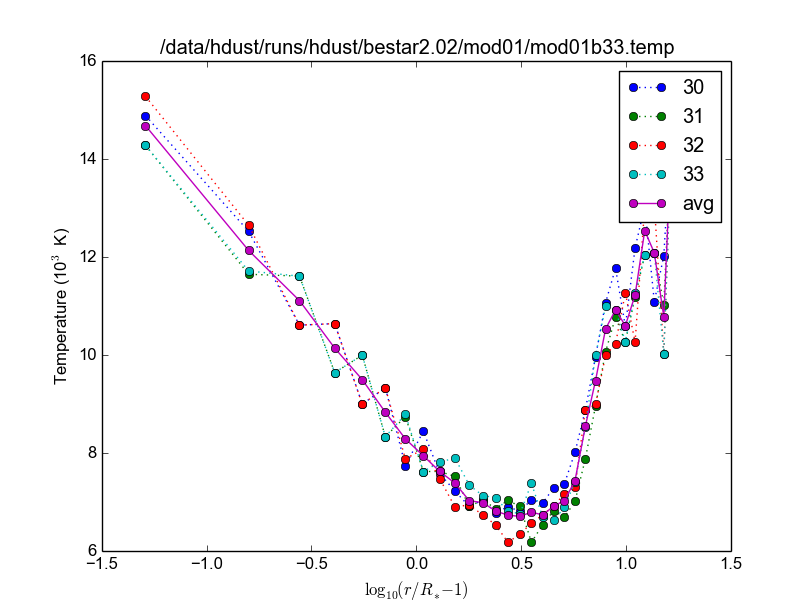
tfile = filenames list.

xax = 0: log10(r/R-1), 1: r/R; 2: 1-R/r

figname = prefix of the output images

fmts = format os the output images.

If interpol==True, what will be plotted is the population along rays of a given latitude. The latitudes are defined in array muplot below.

If interpola==False, what will be plotted is the population for a given mu index as a function of radius, starting with index ncmu/2(midplane) + plus

OUTPUT = …

pyhdust.plottemp2d(tfile, figname=None, fmt=['png'], icphi=0, itype='linear', nimg=128, Rmax=None, trange=None, hres=False)

itype = ‘nearest’, linear’ or ‘cubic’

xax = 0: log10(r/R-1), 1: r/R; 2: 1-R/r

pyhdust.printN0(modn)

Print the n0 of the model inside modn folder. It does a grep of n_0 of all *.txt files of the folder.

Warning: max(M)==14.6Msun (instead of 20.0Msun).

INPUT: string

OUTPUT: figures written.

pyhdust.readSingleBe(sBfile)

Read the singleBe output

OUTPUT = rgrid, lsig_r, nsnaps, simdays, alpha

pyhdust.read_vol_dens_temp(tfile)

Returns the values of volume, dens, temp of tfile.

Example:

>>> tfile = "bestar2.02/mod01/mod01b33.temp"
>>> volume, dens, temp =  read_vol_dens_temp(tfile)
>>> total_mass = np.sum(volume*dens)  # grams (CGS)
>>> avg_temp_by_mass = np.sum(volume*dens*temp) / total_mass
>>> avg_temp_by_vol = np.sum(volume*temp) / np.sum(volume)

pyhdust.readdust(dfile)

Read *.dust files

• ncr = número de células da simulação na coordenada radial

• ncmu = número de células da simulação na coordenada latitudinal

• ncphi = número de células da simulação na coordenada azimutal

• Rstar = raio da estrela (Rsun)

• Ra = raio máximo da simulação, onde acabam todas as poeiras (Rsun)

• pcrc = coordenadas das células em raio

• pcmuc = coordenadas das células em mu

• pcphic = coordenadas das células em phi

• pcr = distância entre as células em raio

• pcmu = distância entre as células em mu

• pcphi = distância entre as células em phi

• ntip = número de tipos de poeira determinados para a simulação

(composição) - na = número de tamanho por tipo da poeira - NdustShells = número de camadas de poeiras da simulação - Rdust = raio onde está(ão) a(s) camada(s) - Tdestruction = temperatura na qual os grãos são evaporados - Tdust = temperatura da poeira numa da posição da grade da simulação (r,phi,mu) - lacentro = controla os tipos e tamanhos das poeiras

pyhdust.readfullsed2(sfile)

Read data from HDUST fullSED2 file.

Parameter

sfile: str

HDUST fullSED2 file path

returns:

• numpy.array – np.array(nobs, nlbd, -1), where the number of columns from fullSED2 file replaces “-1”. Example: lbd_obs0 = fs2data[0, :, 2].

• - 0 (cos(i) == cos(mu))

• - 1 (cos(phi))

• - 2 (lambda)

• - 3 (flux)

• - 4 (sct flux)

• - 5 (emit flux)

• - 6 (trans flux)

• - 7 (Q flux)

• - 8 (U flux (zero for symmetric disks))

pyhdust.readphotxdr(xdrfile='kur_ap00k0.xdr', quiet=False)

doc

pyhdust.readsed2(sfile)

Read data from HDUST SED2 file.

Note: this format is different of readfullsed2.

Parameters:

sfile (str) – HDUST SED2 file path

Return type:

np.array(nobs*nlbd, -1), where number of columns from SED2 file

replaces “-1” :returns: SED2 header info

pyhdust.readtemp(tfile, quiet=False)

Read HDUST temp file

• ncr = número de células da simulação na coordenada radial

• ncmu = número de células da simulação na coordenada latitudinal

• ncphi = número de células da simulação na coordenada azimutal

• nLTE = number of atomic LTE levels

• nNLTE = number of atomic NLTE levels

• beta = flare disk parameter

• Rstar = raio da estrela (Rsun)

• Ra = raio máximo da simulação, onde acabam todas as poeiras (Rsun)

• pcrc = coordenadas das células em raio

• pcmuc = coordenadas das células em mu

• pcphic = coordenadas das células em phi

• pcr = distância entre as células em raio

• pcmu = distância entre as células em mu

• pcphi = distância entre as células em phi

data format is: data[nLTE+6, ncr, ncmu, ncphi]

See also

Temperature are in data[3, …]. More info. see plottemp() function.

Parameters:

sfile (str) – HDUST fullSED2 file path.

Return type:

np.array(nobs, nlbd, -1), number of columns from fullSED2 file replaces “-1”.)

Returns:

HDUST fullSED2 file content.

OUTPUT = ncr,ncmu,ncphi,nLTE,nNLTE,Rstar,Ra,beta,data,pcr,pcmu,pcphi

pyhdust.readtempmass(tfile, quiet=False)

Read HDUST temp file

OUTPUT = mass (in g)

pyhdust.rho2Mdot(Req, alpha, cs, M, rho0, R0)

Equation A.12 Faes (2015)

All values in cgs units!

pyhdust.rho2sig(Req, rho0, cs, M)

Equation A.8, Faes (2015)

All values in cgs units!

pyhdust.sed2info(sfile)

Read info from a HDUST SED2 file.

Parameters:

sfile (str) – HDUST SED2 file path

Return type:

tuple of floats

Returns:

nlbd, nobs, Rstar, Rwind, the HDUST parameters

pyhdust.sig0_to_n0(sig0, M, Req, f, Tp, mu=0.5)

VDD Steady-State conversion between Sigma0 [g/cm2] to n0 ([ionized] particles/volume) .

INPUT: sig0 (float), M, Req (mass and equatorial radius, Solar units), fraction and polar temperature ([0-1], Kelvin) and mu molecular weight [0.5-2.0].

OUTPUT: n0 (particles cm-3)

pyhdust.tefflum_dJN(s, b)

Calculate the Teff and Lum from s and b variables from de Jager & Niewuwenhuijzen (1987).

return log10_T, log10_L (in Solar and Kelvin units)

Spec	s-value	s-step/0.1-Sp
01-09	0.1-0.9	0.1
09-B2	0.9-1.8	0.3
B2-A0	1.8-3.0	0.15
A0-F0	3.0-4.0	0.1
F0-G0	4.0-5.0	0.1
G0-K0	5.0-5.5	0.05
K0-M0	5.5-6.5	0.1
M0-M10	6.5-8.5	0.2

L class	b-value
V	5.0
IV	4.0
III	3.0
II	2.0
Ib	1.4
Iab (or I)	1.0
Ia	0.6
Ia+	0.0

The calcs are made based on Chebyshev polynomials.

pyhdust.temp_interp(tempfile, theta, pos=[0, 1])

Returns temp file properties interpolated at a given line-of-sight

Usage: r, interp = temp_interp(tempfile, theta, pos=[0, 1])

theta = line of sight from midplane, in degrees pos = 0: T [K]

1-25: energy levels population fraction 26: ionization fraction 27: number density [cm-3]